Introduction to programming
for FYS-MEK1110
Milad Hobbi Mobarhan, Svenn-Arne Dragly and Jonas Van den Brink
Week 1
- Motivation and course goals
- Course overview
- Terminal basics
- Python vs MATLAB
- Functions and Plotting
Motivation
- Programming is important in almost every field!
- Important for automating.
- There will be a knowledge gap in the society.
Programming in other courses
- FYS1120: Electromagnetism
- MAT1120: Linear algebra
- AST1100: Introduction to Astrophysics
- Other courses: FYS2130, FYS2140, FYS2160,....
Goals
- To provide a good practical background to preform calculations in Python and MATLAB relevant to FYS-MEK1110.
- You learn programming by doing it, not by just reading how to do it.
Overview
- Terminal basics
- From single commands to a program containing a lot of commands.
- Functions, arrays, plotting
- for, if and while loops
- Euler's algorithm $\rightarrow$ Project: Sliding on snow
Compendium, notes, etc
Terminal Basics

Commands
>> date
Wed Jan  9 17:31:05 CET 2013
Useful Commands
Working directory
>> pwd
/home/milad/documents
List files
>> ls
folder1 folder2
Change working directory
>> cd folder1
>> pwd
/home/milad/documents/folder1
>> cd ..
>> pwd
/home/milad/documents
Make directory/folder
>> mkdir folder3
>> ls
folder1 folder2 folder3
Remove directory/folder
>> rm -r folder3
>> ls
folder1 folder2
Make an empty file
>> touch file
>> ls
folder1 folder2 file
Remove file
>> rm file
>> ls
folder1 folder2
Move files
>> mv name_of_file destination
Copy files
>> cp name_of_file destination
Python vs MATLAB
from pylab import *
n = 1000
x = zeros((n,3))
v = zeros((n,3))
a = zeros((n,3))

m = 1
q = 1

B = array([0,0,1])
omega = q * linalg.norm(B)/m
n = 1000;
x = zeros(n,3);
v = zeros(n,3);
a = zeros(n,3);

m = 1;
q = 1;

B = [0 0 1];
omega = q*norm(B)/m;
Equal qualities
Both are easy to learn
Both are useful for maths and physics
Both give a quick way to do programming
Both are very easy to use
Differences
Python is free
(as in both speech and beer)
MATLAB costs money
MATLAB may be easier to install
Python can be easy
(but it can have a bad day...)
Python is able to do tons of stuff
(from physics and maths to games and applications, using modules...)
MATLAB is more limited
MATLAB comes with a strong editor
Python does not
(but you can install great editors such as Spyder...)
What to choose?
We recommend Python
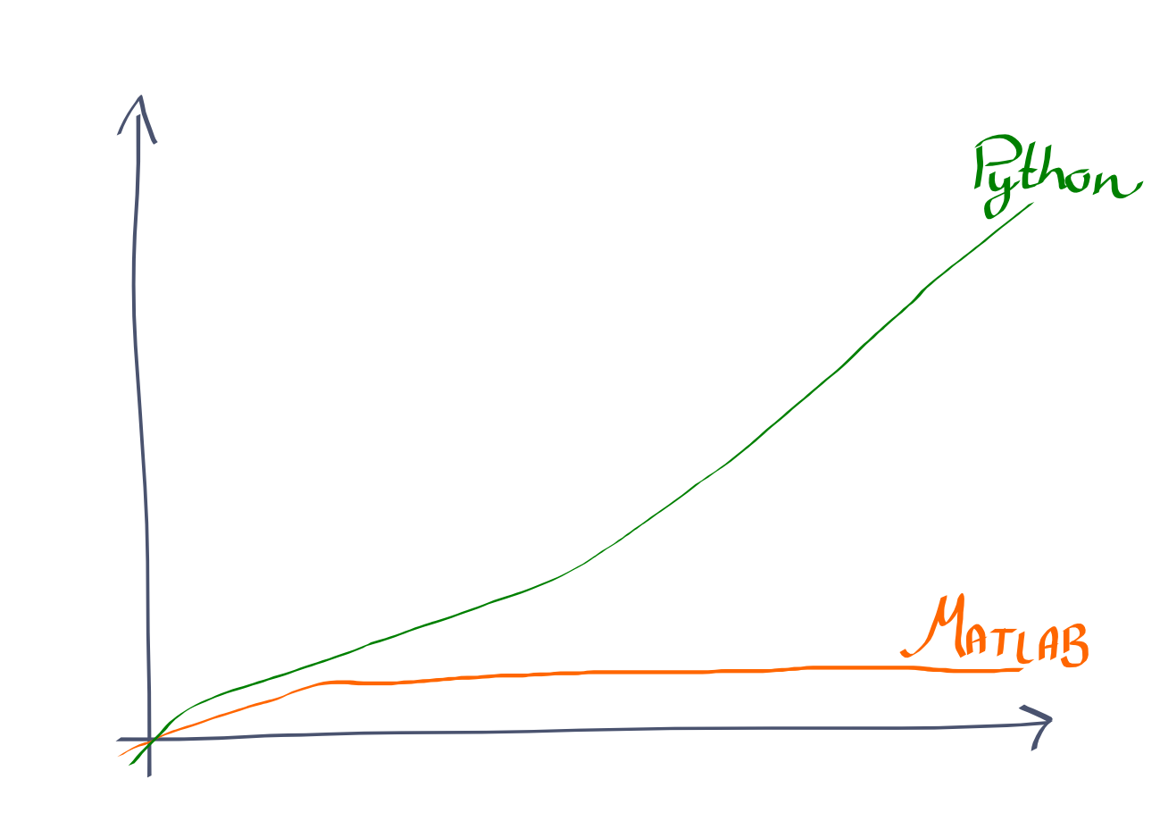
But teach both ;)
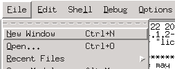
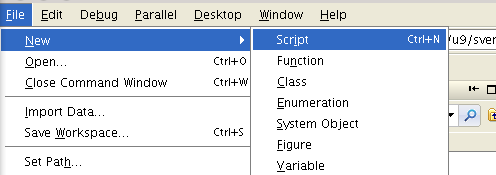
Getting down and dirty
Start your editors!
echo export PATH=/mn/felt/u9/svennard/mayavi/epd-latest/bin/:$PATH >> ~/.bashrc && source ~/.bashrc

idle
matlab
It's a calculator!
>>> 9*4
36
>> 9*4
36
It's a calculator!
>>> 9/5
1
>>> 9./5.
1.8
>> 9/5
1.8
Maths
>>> from pylab import *
>>> 4*pi
12.566370614359172
>> 4*pi
12.567
Variables
>>> TC = 40.
>>> print TC
40.0
>> TC = 40
40
>> TC
40
Temperature conversion
>>> TF = 9./5. * TC + 32.
>>> print TF
104.0
>> TF = 9/5 * TC + 32
104
Changing variable values
>>> TC = 12.
>>> print TC
12.0
>>> print TF
104.0
>> TC = 12
12
>> TF
104
Ooops! What went wrong?
Push the ↑ button on your keyboard a couple of times and calculate TF again...
Scripting
Python
MATLAB
Temperature conversion script
TC = 12.
TF = 9./5. * TC + 32.
print TF
TC = 12;
TF = 9/5 * TC + 32;
Run with F5.
(Note the semicolons for MATLAB...)
Testing behaviour
Type a new value for TC on the command line and re-run the script. Did anything change?
Functions
Temperature conversion function
def convertF(TC):
    TF = 9./5.*TC + 32.
    return TF

# different ways of printing
print convertF(10)
TF = convertF(30)
print TF
MATLAB
convertF.m
function TF=convertF(TC);
TF = 9/5*TC + 32;
return
main.m
% different ways of printing
convertF(10)
TF = convertF(30);
TF
Arrays
>>> TC = array([0, 10, 15.5, 20])
>>> print TC
[  0.   10.   15.5  20. ]
MATLAB
>> TC = [0 10 15.5 20]
TC =

         0   10.0000   15.5000   20.0000
Arrays and functions
>>> TC = array([0, 10, 15.5, 20])
>>> print convertF(TC)
[ 32.   50.   59.9  68. ]
MATLAB
>> TC = [0 10 15.5 20];
>> convertF(TC)

ans =

   32.0000   50.0000   59.9000   68.0000
Plotting
Plotting
Python
>>> m = [1, 2, 4, 6, 9, 11]
>>> V = [0.13, 0.26, 0.50, 0.77, 1.15, 1.36]
>>> print V[3]
0.77
>>> plot(m,V,'o')
>>> xlabel('m [kg]')
>>> ylabel('V [l]')
>>> show()


>>> m = [1, 2, 4, 6, 9, 11]
>>> V = [0.13, 0.26, 0.50, 0.77, 1.15, 1.36]
>>> print V[3]
0.77
>>> plot(m,V,'o')
>>> xlabel('m [kg]')
>>> ylabel('V [l]')
>>> show()
>>> m = [1, 2, 4, 6, 9, 11]
>>> V = [0.13, 0.26, 0.50, 0.77, 1.15, 1.36]
>>> print V[3]
0.77
>>> plot(m,V,'o')
>>> xlabel('m [kg]')
>>> ylabel('V [l]')
>>> show()
>>> m = [1, 2, 4, 6, 9, 11]
>>> V = [0.13, 0.26, 0.50, 0.77, 1.15, 1.36]
>>> print V[3]
0.77
>>> plot(m,V,'o')
>>> xlabel('m [kg]')
>>> ylabel('V [l]')
>>> show()
MATLAB
>> m = [1 2 4 6 9 11];
>> V = [0.13 0.26 0.50 0.77 1.15 1.36];
>> V(4)
ans =     0.7700
>> plot(m,V,'o')
>> xlabel('m [kg]')
>> ylabel('V [l]')
Exercises
Here are some exercises you can do:
1.1, 1.2, 1.3, 1.6
Week 2
- Quick repetition from last week
- for-loops
- if-tests
Compendium, notes, etc
Reptition
Start your editors!
echo export PATH=/mn/felt/u9/svennard/mayavi/epd-latest/bin/:$PATH >> ~/.bashrc && source ~/.bashrc

idle
matlab
It's a calculator!
>>> 9*4
36
>> 9*4
36
>>> 9/5
1
>>> 9./5.
1.8
>> 9/5
1.8
Maths
>>> from pylab import *
>>> 4*pi
12.566370614359172
>> 4*pi
12.567
Temperature conversion
>>> TC = 40.
>>> print TC
40.0
>>> TF = 9./5. * TC + 32.
>>> print TF
104.0
>> TC = 40
40
>> TC
40
>> TF = 9/5 * TC + 32
104
Changing variable values
>>> TC = 12.
>>> print TC
12.0
>>> print TF
104.0
>> TC = 12
12
>> TF
104
Ooops! What went wrong?
Push the ↑ button on your keyboard a couple of times and calculate TF again...
Reptition
Scripting
Python
MATLAB
Temperature conversion function
def convertF(TC):
    TF = 9./5.*TC + 32.
    return TF
MATLAB
convertF.m
function TF=convertF(TC);
TF = 9/5*TC + 32;
return
>>> print convertF(40)
104.0
MATLAB
>> convertF(40)
104.0
Run with F5.
(Note the semicolons for MATLAB...)
Reptition
Arrays
>>> TC = array([0, 10, 15.5, 20])
>>> print TC
[  0.   10.   15.5  20. ]
MATLAB
>> TC = [0 10 15.5 20]
TC =

         0   10.0000   15.5000   20.0000
Arrays and functions
>>> TC = array([0, 10, 15.5, 20])
>>> print convertF(TC)
[ 32.   50.   59.9  68. ]
MATLAB
>> TC = [0 10 15.5 20];
>> convertF(TC)

ans =

   32.0000   50.0000   59.9000   68.0000
Plotting
Python
>>> m = [1, 2, 4, 6, 9, 11]
>>> V = [0.13, 0.26, 0.50, 0.77, 1.15, 1.36]
>>> print V[3]
0.77
>>> plot(m,V,'o')
>>> xlabel('m [kg]')
>>> ylabel('V [l]')
>>> show()
MATLAB
>> m = [1 2 4 6 9 11];
>> V = [0.13 0.26 0.50 0.77 1.15 1.36];
>> V(4)
ans =     0.7700
>> plot(m,V,'o')
>> xlabel('m [kg]')
>> ylabel('V [l]')
This is what we are going to do today!
and here is all the code we need
from pylab import *
from time import sleep
ion()
line, = plot(0,0)
xlim(-4,4)
ylim(-4,4)
show()
for maxt in arange(-50,50,0.2):
    t = arange(-50,maxt,0.01)
    x = sin(t) * (exp(cos(t)) - 2*cos(4*t) - pow(sin(t/12.), 5))
    y = cos(t) * (exp(cos(t)) - 2*cos(4*t) - pow(sin(t/12.), 5))
    line.set_xdata(x)
    line.set_ydata(y)
    draw()
    sleep(0.01)
Don't worry, we'll explain it all to you ;)
Why for loops?
for-loops
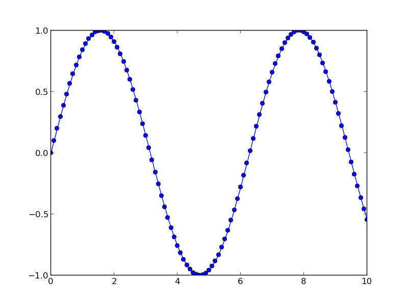
Let's say you want to plot
$f(x)=sin(x)$ for
$x=0, 0.1, 0.2, 0.3, ...9.9, 10$
We need to make an array which is a list of all x-values
It would be really boring to type every element in this array!
>>> x = array([0, 0.1, 0.2, 0.3])
MATLAB
>> x = [0, 0.1, 0.2, 0.3]
Fortunately, there is a more efficient way of doing this:
by using a for-loop!
Going from $0.0$ to $10.0$ in steps of $0.1$ we need:
zeros((n,m)) function:
makes an array with dimention $n \times m$, where all elements are zero.
>>> zeros((1,10))
array([[ 0.,  0.,  0.,  0.,  0.,  0.,  0.,  0.,  0.,  0.]])

>>> zeros((10,1))
array([[ 0.],
       [ 0.],
       [ 0.],
       [ 0.],
       [ 0.],
       [ 0.],
       [ 0.],
       [ 0.],
       [ 0.],
       [ 0.]])
for-loop:
from pylab import *
x0 = 0.0
x1 = 10.0
dx = 0.1


n = ceil (( x1 - x0 ) / dx ) + 1

x = zeros (( n , 1) )

for i in range (int (n)) :
    x [ i ] = x0 + i * dx

plot (x , sin(x),'-o' )
show ()
print x, n
range-function
>>> range(10)
[0, 1, 2, 3, 4, 5, 6, 7, 8, 9]

>>> range(0,10)
[0, 1, 2, 3, 4, 5, 6, 7, 8, 9]

>>> range(1,10)
[1, 2, 3, 4, 5, 6, 7, 8, 9]

>>> range(1,10,1)
[1, 2, 3, 4, 5, 6, 7, 8, 9]

>>> range(1,10,2)
[1, 3, 5, 7, 9]
>>> range(0,10,0.1)
Vectorization
linspace(a,b,c)
>>> linspace(1,10,10)
array([  1.,   2.,   3.,   4.,   5.,   6.,   7.,   8.,   9.,  10.])
from pylab import *
x=linspace(0,10,100)
plot (x , sin(x),'-o' )
show ()
arange(a,b,c)
>>> arange(0,1,0.1)
array([ 0. ,  0.1,  0.2,  0.3,  0.4,  0.5,  0.6,  0.7,  0.8,  0.9])
from pylab import *
x=arange(0,10,0.1)
plot (x , sin(x),'-o' )
show ()
Back to the butterfly!
from pylab import *
from time import sleep
ion()
line, = plot(0,0)
xlim(-4,4)
ylim(-4,4)
show()
for maxt in arange(-50,50,0.2):
    t = arange(-50,maxt,0.01)
    x = sin(t) * (exp(cos(t)) - 2*cos(4*t) - pow(sin(t/12.), 5))
    y = cos(t) * (exp(cos(t)) - 2*cos(4*t) - pow(sin(t/12.), 5))
    line.set_xdata(x)
    line.set_ydata(y)
    draw()
    sleep(0.01)
What if...
...we explore if-tests?
Dice throwing
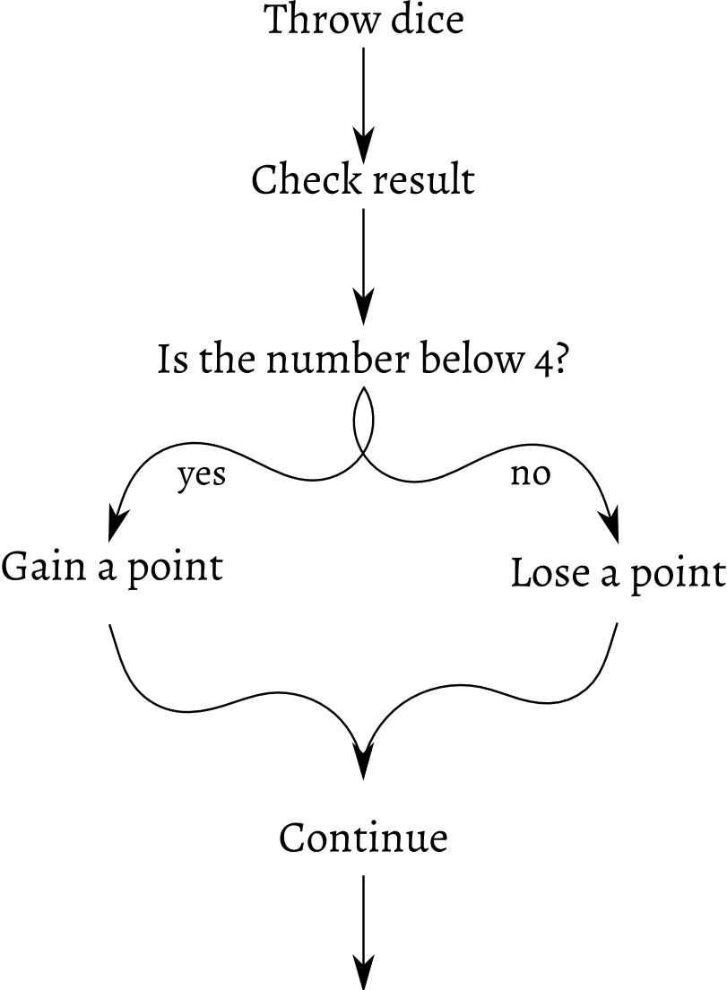
Dice throwing
from pylab import *
points = 0
diceResult = randint(1,7)
if diceResult < 4:
    points = points + 1
else:
    points = points - 1
print points
Dice throwing
from pylab import *
points = 0
for i in range(1000):
    diceResult = randint(1,7)
    if diceResult < 4:
        points = points + 1
    else:
        points = points - 1
print points
Week 3
- Euler's method
Programming motion
Taking positions of objects through steps in time
Programming motion
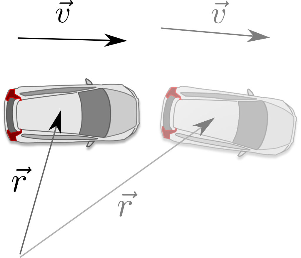
Programming motion
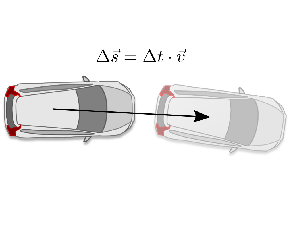


$\Delta a = 0$
$\Delta v = \overline{a} \cdot \Delta t$
$\Delta x = \overline{v} \cdot \Delta t$
$\vec r(t_i + \Delta t) = \vec r(t_i) + \Delta t \cdot \vec v(t_i)$
$\vec v(t_i + \Delta t) = \vec v(t_i) + \Delta t \cdot \vec a(t_i)$
Python example
from pylab import *
n = 100
dt = 0.10
x = zeros((n,1))
v = zeros((n,1))
a = zeros((n,1))
t = zeros((n,1))
a[0] = 300
x[0] = 0
v[0] = 0
for i in range(0,n-1):
   a[i+1] = a[i]
   v[i+1] = v[i] + a[i]*dt
   x[i+1] = x[i] + v[i+1]*dt
   t[i+1] = t[i] + dt
subplot(3,1,1)
plot(t,a)
xlabel('t')
ylabel('a')
subplot(3,1,2)
plot(t,v)
xlabel('t')
ylabel('v')
subplot(3,1,3)
plot(t,x)
xlabel('t')
ylabel('x')